To show true and false more clearly, blue variable below means true and red means false.

SAT: Satisfiability

Basis

Literal: a variable $x$ and its negation

Clause: a disjunction of literals, like: $x\vee\neg y$

Boolean Assignment: a mapping of variables to Boolean values.

SAT: Constraint satisfaction problem on a set of clauses.

• Given a set of clauses, find a Boolean assignment that makes all clauses true.

The SAT problems are always defined by Conjunctive Normal Form. Any propositional logic formula can be expressed in Conjunctive Normal Form.

Methods

Basic Method: Brute-Force

Sat(assign) {
    if (assign is complete) {
        if (at least one literal is true in each clause)
            return true
        else
            return false
    }
    else {
        choose a variable x that has not been assigned
        return Sat(assign U {x=true}) || Sat(assign U {x=false})
    }
}

Optimization 1: Conflict Detection

This method detect conflict when assigning variables to reduce useless route.

Sat(assign) {
    if (assign has conflict) return false
    if (assign is complete) return true
    return Sat(assign U {x=true}) || Sat(assign U {x=false})
}

Optimization 2: DPLL

DPLL stands for Davis-Putnam-Logemann-Loveland method, which using Assignment Propagation method and Conflict Detection together. Assignment Propagation is what we want to introduce now. This method propagate the value of other literal with current assignment.

Common Propagation Rules

• Unit Propagation: The only unassigned literal must be true if other literals are all false in a clause.

  {-1, 2, 3} ⇒ 3

• Unate Propagation: If a clause contains at least one True literal, it could be deleted. As the value of other literal would not influence the result of this clause.

• Pure Literal Propagation: If a variable has only one format in all clauses, we can let the literal contains it be true forever. Then all the clauses contain it could be deleted.

  {-1, 2 ,3} {-1, -2, 3} {-1, 3, 4}

DPLL(assign) {
    assignx = propagation(assign)
    if (assignx has conflict) return false
    if (assignx is complete) return true
    return DPLL(assignx U {x=true}) || DPLL(assignx U {x=false})
}

High-level Propagation

• Probing: If x=0 and x=1 can both lead to y=1, then y could be propagated as 1.
• Equivalence Classes: Check the equivalence clauses and keep only one of them.

Notice! In some conditions, propagation might be slower and more inefficient than the basic Brute-Force, so it should be discussed in procedure whether to do the propagation.

Optimization 3: Branching Heuristics

The choice which variable is assigned first could influence efficiency largely. Take the clauses below as an example. If we choose to assign 1 or 2 first, we could find out they could not be satisfied rapidly. But if we choose 3-8, we need to perform several iterations.

• {1, -2} {1, 2} {-1, -2} {-1, 2} {3, 4, 5, 6, 7, 8}

Then we introduce Branching Heuristics

Based on clause set:

• Select variables in the shortest clauses.
• Select variables that appear most frequently.

Based on historical data:

• Select variables that have previously caused conflicts.

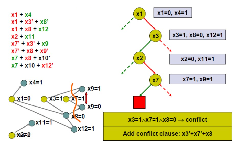
Optimization 4: CDCL

CDCL stands for Conflict-Driven Clause Learning. When facing new conflict, the solver will learn the new conflict as a new constraint. This process is called Clause Learning.

Note that the iteration starting from the newly added constraints actually ensures that previously explored conflicting assignments will not occur.

• Therefore, there is no need to record the assignments that have been traversed before; you can simply choose any remaining variable and assignment each time.
• Deriving a conflict from an empty assignment means UNSAT.

Example:

cdcl() {
    assign = new Assignment
    while (true) {
        assignx = propagation(assign)
        if (assignx has conflict) {
            if (assign is None) return false;
            addNewConstraint()
            assign.undoAssignment()
        }
        else {
            if (assignx is complete) return true;
            select a unassigned variable, let it be true of false
            add it to assign
        }
    }
}

Optimization 4.1: VSIDS

VSIDS stands for Variable State Independent Decaying Sum.

• Score all variables based on the frequency they appear.
• Add points to the variables in a clause when a new clause is added.
• Divide the score of all variables by a constant every once in a while.

SMT: Satisfiability Modulo Theories

Basis

SAT solves whether a propositional logic formula is satisfiable, which looks like $A\vee B\wedge \neg C$. While formulas in real life may look like $a+bb$. Many symbols are not contained in the logical system, making the formula impossible to do deductions.

Theory: Theory is used to assign meanings to these types of symbols. A theory consists of a set of axioms and the conclusions that can be derived from these axioms.

SMT: Given a set of theories, finding the satisfiability of this set of theories.

EUP (Equality with Uninterpreted Functions)

EUP is a common theory. The axioms it contained is showed below:

• $a=b \Rightarrow f(a)=f(b)$
• $a=b\Leftrightarrow \neg(a\ne b)$

Eager Method

Transform the SMT problem into a SAT problem, then solve it with the SAT solver

The example is complex, imagine by yourself……

Problems of Eager Method:

• Many theories have specialized solving algorithms, such as: EUF (Equality with Uninterpreted Functions) can be solved using a fixed-point algorithm that continuously merges equivalence classes. After being encoded into SAT, SAT solvers cannot take advantage of these algorithms.
• The modularity is not high. Each theory requires a separate encoding method. When using different theories together, it is necessary to ensure that the encoding methods are compatible.

Lazy Method

A black-box containing SAT solver and each kind of theory solver. Here is an example how Lazy Method solve a problem.

• Encode these constrains, let 1 be the first formula and -2 be the second formula and so on. (For inequation, we commonly do NOR for it) Then the problem above could be transformed into clauses: {1}, {-2, 3}, {-4}

• The SAT solver returns a result SAT and an assignment {1, 2, 4}

• Turn the assignment into formula and put into the EUF solver:

  $\{g(a)=c ,\ f(g(a)) \neq f(c) ,\ c \neq d\}$

• EUF solver returns UNSAT

• Do clause learning. The input of SAT solver will be {1}, {-2, 3}, {-4}, {-1, 2, 4}

• The SAT solver returns SAT and an assignment {1, 2, 3, 4}

• EUF solver returns UNSAT

• Do clause learning. The input of SAT solver will be {1}, {-2, 3}, {-4}, {-1, 2, 4}, {-1, -2, -3, 4}

• SAT solver returns UNSAT

Problems of Lazy Method:

Think about the example below, the EUF solver could tell that {1}, {-4} has conflict directly. But SAT solver do not have such knowledge. This could lead to useless iteration. So we think about adding interface to theory solver which could let SAT know other information as what we have done in CDCL.

DPLL(T)

Interface Function

propagation:

• Input: a set of formulas and known Ture or False of some formulas
• Output: formulas in this set that could be propagated

get_unsatisfiable_core:

• Input: a set of formulas with known conflict
• Output: the minimum sub set of these formulas that still cause the conflict

Core Algorithm

Break the SAT black box by integrating theoretical solvers centered around the CDCL.

dpll_t() {
    assign = new Assignment
    while (true) {
        if (!check(assign)) {
            if (assign is None) return false;
            addNewConstraint();
            assign.undoAssignment()
        }
        else {
            if (assignx is complete) return true;
            select a unassigned variable, let it be true of false
            add it to assign
        }
    }
}

check(assign) {
    do {
        assignx = propagation(assign);
        if(assignx has conflict) return false;
        if(TheorySolver(assignx) = UNSAT) return false;
        assignx = TheorySolverPropagation(assign);
        if(assignx has conflict) return false;
    } while(assignx != assign)
    return true;
}

addNewConstrain() {
    if(conflict in propagation) ConflictSet = Predecessor of the conflict clause.;
    else ConflictSet = TheorySolver.get_unsatisfiable_core();
    add(NOR(ConflictSet));
}

Example:

Transform it into clauses: {1}, {-2, 3}, {-4, 5}

Clauses	Assignment	Propagation	Method
{1}{-2, 3}{-4, 5}	{}	{1}	Unit Propagation
{1}{-2, 3}{-4, 5}	{}	{1, 2}	T-Propagation
{1}{-2, 3}{-4, 5}	{}	{1, 2, 3}	Unit Propagation
{1}{-2, 3}{-4, 5}	{-4}	conflict set: {1, 3, -4}	T-Solver UNSAT
{1}{-2, 3}{-4, 5}{-1, -3, 4}	{}	{1, 2, 3, 4, 5}	Unit Propagation

Nelson-Oppen Method

This method is used to combine different theory solvers in a modular way. It ensures that the combined solution respects the individual theory constraints while solving the overall SMT problem.